At this year’s Minds Mastering Machines (M3) conference in Karlsruhe, the focus was on best practices for GenAI, RAG systems, case studies from different industries, agent systems, and LLM, as well as legal aspects of ML. We gave three talks about our projects.
In modern higher education, the optimisation and personalisation of the learning process is extremely important. Technologies such as Large Language Models (LLMs) and Retrieval Augmented Generation (RAG) can play a supporting role, especially in complex courses such as law. A pilot project at the University of Leipzig, involving the university’s Computing Centre and the Faculty of Law, shows how these technologies can be successfully used in the form of an AI chatbot.
Background and Turing
In 1950, Alan Turing posed the revolutionary question in his essay “Computing Machinery and Intelligence”: Can machines think? He proposed the famous “imitation game”, now known as the Turing Test. In his view, a machine could be said to “think” if it could fool a human tester.
This idea forms the theoretical basis for many modern AI applications. We have come a long way since then, and new opportunities are opening up for students in particular to use AI tools such as LLMs to support their studies.
How does such a chatbot work for law studies?
The AI-based chatbot uses OpenAI’s advanced language models, called Transformers. These systems, such as GPT-4, can be augmented with the Retrieval Augmented Generation (RAG) method to provide correct answers to more complex legal questions. The process consists of several steps:
1. Ask a question (Query): Students ask a legal question, for example, “What is the difference between a mortgage and a security mortgage?”
2. Processing the query (Embedding): The question is converted into vectors so that it can be read and analysed by the LLM.
3. Search in vector database: The retrieval system searches a vector database for relevant texts that match the question. These can be lecture notes, case solutions or lecture slides.
4. Answer generation: The LLM analyses the data found and provides a precise answer. The answer can be provided with references, e.g. the page in the script or the corresponding slide in the lecture.
This is a powerful tool for law students, as they not only get quick answers to very individual questions, but also have direct links to the relevant teaching materials. This makes it easier to understand complex legal concepts and encourages independent learning.
Benefits for students and professors
Chatbots offer several benefits for teaching and learning in universities. For students, this means
Personalised learning support: Students can ask individual questions and receive tailor-made answers.
Adaptation to different subjects: You can easily adapt the chatbot to different areas of law, such as civil, criminal or public law. It can also explain more difficult legal concepts or help with exam preparation.
Flexibility and cost transparency: Whether at home or on the move, the chatbot is always available and provides access to key information – via a Learning Management System (LMS) such as Moodle or directly as an app. In addition, monthly token budgets ensure clear cost control.
The use of LLMs in combination with RAG also has advantages for teachers:
Planning support: AI tools can help to better structure courses.
Development of teaching materials: AI can support the creation of assignments, teaching materials, case studies or exam questions.
Challenges in using LLMs
Despite the many benefits and opportunities offered by chatbots and other AI-based learning systems, there are also challenges that need to be considered:
Resource-intensive: The operation of such systems requires a high level of computing power and costs.
Provider dependency: Currently, many such systems rely on interfaces to external providers such as Microsoft Azure or OpenAI, which can limit independence from universities.
Quality of answers: AI systems do not always produce correct results. “Hallucinations (incorrect or nonsensical answers) can occur. Like all data-based systems, LLMs can be biased by the training data used. Therefore, both the accuracy of the answers and the avoidance of bias must be ensured.
The technical background: Azure and OpenAI
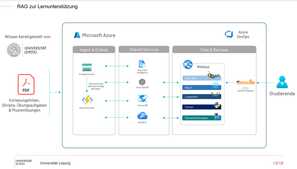
The chatbot above is built on the Microsoft Azure cloud infrastructure. Azure provides several services that enable secure and efficient computing. These include:
AI Search: A hybrid search that combines both vector and full-text search to quickly find relevant data.
Document Intelligence: Extracts information from PDF documents and provides direct access to lecture slides, scripts, or other educational materials.
OpenAI: Azure provides access to OpenAI’s powerful language models. For example, the implementation uses GPT-4 Turbo and the ada-002 model for text embeddings to efficiently generate correct answers.
Presentation of the data processing procedure
Conclusion
The pilot project with the University of Leipzig shows how the use of LLMs and RAGs can support higher education. These technologies not only make learning processes more efficient, but also more flexible and targeted.
The use of Microsoft Azure also ensures secure and GDPR-compliant data processing.
The combination of powerful language models and innovative search methods offers both students and teachers new and effective ways to improve learning and teaching. The future of learning will be personalized, scalable, and always available.
https://www.scieneers.de/wp-content/uploads/2024/11/aa.jpg413744Florence Lopezhttps://www.scieneers.de/wp-content/uploads/2020/04/scieneers-gradient.pngFlorence Lopez2024-11-08 09:55:022024-12-12 16:25:16How students can benefit from LLMs and chatbots
In many companies, the issue isn’t a lack of data but how to manage and make it accessible to employees. One particularly pressing challenge is the transfer of knowledge from senior employees to younger generations. This is no small task, as it’s not just about transferring what’s documented in manuals or process guides, but the implicit knowledge that exists “between the lines”—the insights and experience locked within the minds of long-serving employees.
This challenge has been present across industries for many years, and as technology evolves, so do the solutions. With the rapid advancement of Artificial Intelligence (AI), particularly Generative AI, new possibilities for preserving and sharing this valuable company knowledge are emerging.
The Rise of Generative AI
Generative AI, especially Large Language Models (LLMs) such as OpenAI’s GPT-4o, Anthropic’s Claude 3.5 Sonnet, or Meta’s Llama3.2, offer new ways to process and make large amounts of unstructured data accessible. These models enable users to interact with company data via chatbot applications, making knowledge transfer more dynamic and user-friendly.
But the question remains — how do we make the right data accessible to the chatbot in the first place? This is where Retrieval-Augmented Generation (RAG) comes into play.
Retrieval-Augmented Generation (RAG) for Textual Data
RAG has proven to be a reliable solution for handling textual data. The concept is straightforward: all available company data is chunked and stored in (vector) databases, where it is transformed into numerical embeddings. When a user makes a query, the system searches for relevant data chunks by comparing the query’s embedding with the stored data.
With this method, there’s no need to fine-tune LLMs. Instead, relevant data is retrieved and appended to the user’s query in the prompt, ensuring that the chatbot’s responses are based on the company’s specific data. This approach works effectively for all types of textual data, including PDFs, webpages, and even image-embedded documents using multi-modal embeddings.
In this way, company knowledge stored in documents becomes easily accessible to employees, customers, or other stakeholders via AI-powered chatbots.
Extending RAG to Video Data
While RAG works well for text-based knowledge, it doesn’t fully address the challenge of more complex, process-based tasks that are often better demonstrated visually. For tasks like machine maintenance, where it’s difficult to capture everything through written instructions alone, video tutorials provide a practical solution without the need for time-consuming documentation-writing.
Videos offer a rich source of implicit knowledge, capturing processes step-by-step with commentary. However, unlike text, automatically describing a video is far from a straightforward task. Even humans approach this differently, often focusing on varying aspects of the same video based on their perspective, expertise, or goals. This variability highlights the challenge of extracting complete and consistent information from video data.
Breaking Down Video Data
To make knowledge captured in videos accessible to users via a chatbot, our goal must be to provide a structured process to convert videos into textual form that prioritizes extracting as much relevant information as possible. Videos consist of three primary components:
Metadata: The handling of metadata is typically straightforward, as it is often available in structured textual form.
Audio: Audio can be transcribed into text using speech-to-text (STT) models like OpenAI’s Whisper. For industry-specific contexts, it’s also possible to enhance accuracy by incorporating custom terminology into these models.
Frames (visuals): The real challenge lies in integrating the frames (visuals) with the audio transcription in a meaningful way. Both components are interdependent — frames often lack context without audio explanations, and vice versa.
Tackling the Challenges of Video Descriptions
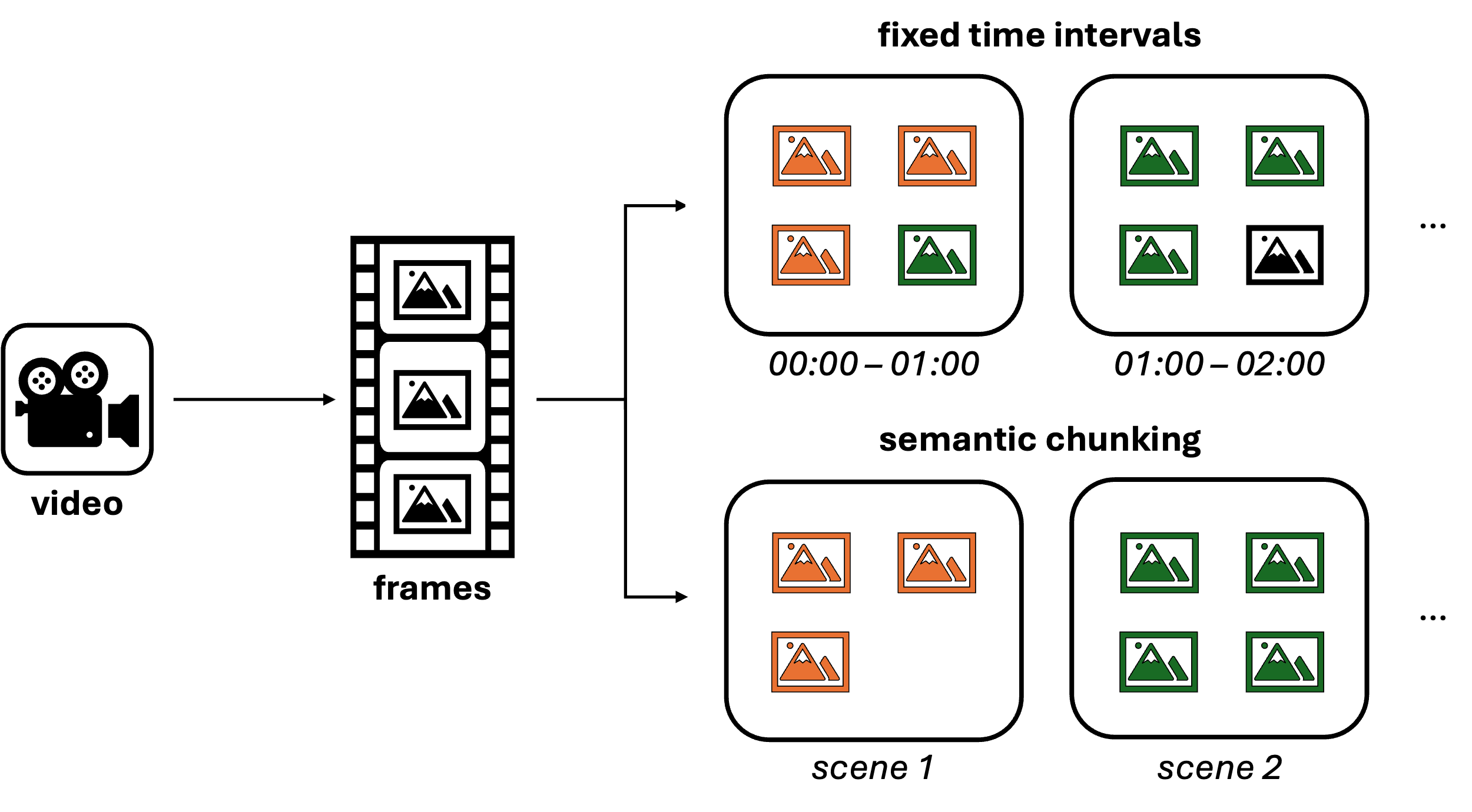
Figure 1: Chunking Process of VideoRAG.
When working with video data, we encounter three primary challenges:
Describing individual images (frames).
Maintaining context, as not every frame is independently relevant.
Integrating the audio transcription for a more complete understanding of the video content.
To address these, multi-modal models like GPT-4o, capable of processing both text and images, can be employed. By using both video frames and transcribed audio as inputs to these models, we can generate a comprehensive description of video segments.
However, maintaining context between individual frames is crucial, and this is where frame grouping (often also referred to as chunking) becomes important. There are two primary methods for grouping frames:
Fixed Time Intervals: A straightforward approach where consecutive frames are grouped based on predefined time spans. This method is easy to implement and works well for many use cases.
Semantic Chunking: A more sophisticated approach where frames are grouped based on their visual or contextual similarity, effectively organizing them into scenes. There are various ways to implement semantic chunking, such as using Convolutional Neural Networks (CNNs) to calculate frame similarity or leveraging multi-modal models like GPT-4o for pre-processing. By defining a threshold for similarity, you can group related frames to better capture the essence of each scene.
Once frames are grouped, they can be combined into image grids. This technique allows the model to understand the relation and sequence between different frames, preserving the video’s narrative structure.
The choice between fixed time intervals and semantic chunking depends on the specific requirements of the use case. In our experience, fixed intervals are often sufficient for most scenarios. Although semantic chunking better captures the underlying semantics of the video, it requires tuning several hyperparameters and can be more resource-intensive, as each use case may require a unique configuration.
With the growing capabilities of LLMs and increasing context windows, one might be tempted to pass all frames to the model in a single call. However, this approach should be used cautiously. Passing too much information at once can overwhelm the model, causing it to miss crucial details. Additionally, current LLMs are constrained by their output token limits (e.g., GPT-4o allows 4096 tokens), which further emphasizes the need for thoughtful processing and framing strategies.
Building Video Descriptions with Multi-Modal Models
Figure 2: Ingestion Pipeline of VideoRAG.
Once the frames are grouped and paired with their corresponding audio transcription, the multi-modal model can be prompted to generate descriptions of these chunks of the video. To maintain continuity, descriptions from earlier parts of the video can be passed to later sections, creating a coherent flow as shown in Figure 2. At the end, you’ll have descriptions for each part of the video that can be stored in a knowledge base alongside timestamps for easy reference.
Bringing VideoRAG to Life
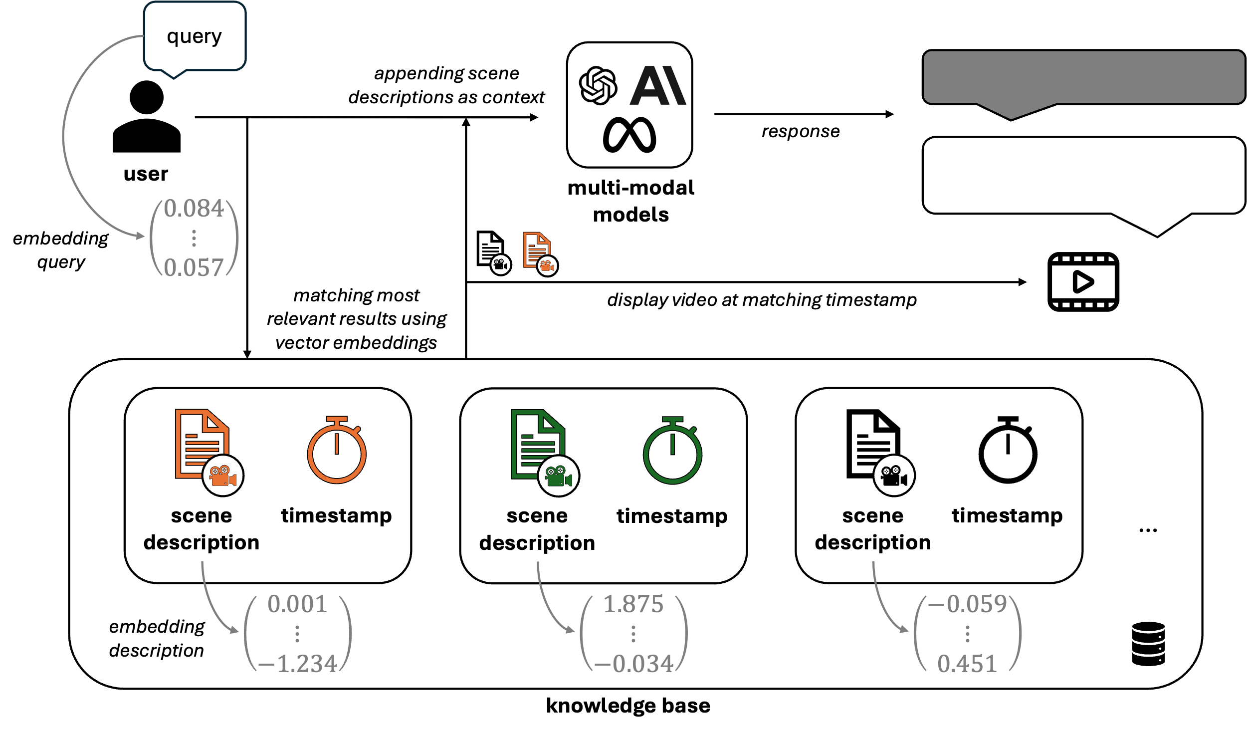
Figure 3: Retrieval process of VideoRAG.
As shown in Figure 3, all scene descriptions from the videos stored in the knowledge base are converted into numerical embeddings. This allows user queries to be similarly embedded, enabling efficient retrieval of relevant video scenes through vector similarity (e.g., cosine similarity). Once the most relevant scenes are identified, their corresponding descriptions are added to the prompt, providing the LLM with context grounded in the actual video content. In addition to the generated response, the system retrieves the associated timestamps and video segments, enabling users to review and validate the information directly from the source material.
By combining RAG techniques with video processing capabilities, companies can build a comprehensive knowledge base that includes both textual and video data. Employees, especially newer ones, can quickly access critical insights from older colleagues — whether documented or demonstrated on video — making knowledge transfer more efficient.
Lessons Learned
During the development of VideoRAG, we encountered several key insights that could benefit future projects in this domain. Here are some of the most important lessons learned:
1. Optimizing Prompts with the CO-STAR Framework
As is the case with most applications involving LLMs, prompt engineering proved to be a critical component of our success. Crafting precise, contextually aware prompts significantly impacts the model’s performance and output quality. We found that using the CO-STAR framework — a structure emphasizing Context, Objective, Style, Tone, Audience, and Response—provided a robust guide for prompt design.
By systematically addressing each element of CO-STAR, we ensured consistency in responses, especially in terms of description format. Prompting with this structure enabled us to deliver more reliable and tailored results, minimizing ambiguities in video descriptions.
2. Implementing Guardrail Checks to Prevent Hallucinations
One of the more challenging aspects of working with LLMs is managing their tendency to generate answers, even when no relevant information exists in the knowledge base. When a query falls outside of the available data, LLMs may resort to hallucinating or using their implicit knowledge—often resulting in inaccurate or incomplete responses.
To mitigate this risk, we introduced an additional verification step. Before answering a user query, we let the model evaluate the relevance of each retrieved chunk from the knowledge base. If none of the retrieved data can reasonably answer the query, the model is instructed not to proceed. This strategy acts as a guardrail, preventing unsupported or factually incorrect answers and ensuring that only relevant, grounded information is used. This method is particularly effective for maintaining the integrity of responses when the knowledge base lacks information on certain topics.
3. Handling Industry-Specific Terminology during Transcription
Another critical observation was the difficulty SST models had when dealing with industry-specific terms. These terms, which often include company names, technical jargon, machine specifications, and codes, are essential for accurate retrieval and transcription. Unfortunately, they are frequently misunderstood or transcribed incorrectly, which can lead to ineffective searches or responses.
To address this issue, we created a curated collection of industry-specific terms relevant to our use case. By incorporating these terms into the model’s prompts, we were able to significantly improve the transcription quality and the accuracy of responses. For instance, OpenAI’s Whisper model supports the inclusion of domain-specific terminology, allowing us to guide the transcription process more effectively and ensure that key technical details were preserved.
Conclusion
VideoRAG represents the next step in leveraging generative AI for knowledge transfer, particularly in industries where hands-on tasks require more than just text to explain. By combining multi-modal models and RAG techniques, companies can preserve and share both explicit and implicit knowledge effectively across generations of employees.
https://www.scieneers.de/wp-content/uploads/2024/10/neu.jpg7581024Arne Grobrueggehttps://www.scieneers.de/wp-content/uploads/2020/04/scieneers-gradient.pngArne Grobruegge2024-10-23 09:14:322025-01-31 13:51:20Leveraging VideoRAG for Company Knowledge Transfer