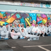
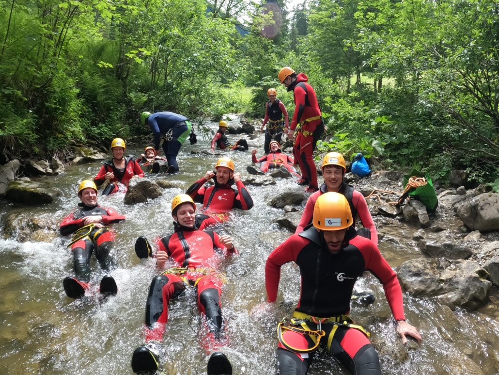
Throwback to our spring event 2025
Most of our colleagues from our three locations Karlsruhe, Cologne, and Hamburg met in Hamburg for two days. We discussed specialist and internal topics, gained new ideas, and shared experiences.

technology content
Most of our colleagues from our three locations Karlsruhe, Cologne, and Hamburg met in Hamburg for two days. We discussed specialist and internal topics, gained new ideas, and shared experiences.

After giving an overview of Real-Time Intelligence in Microsoft Fabric in the previous article, today we’ll dive a bit deeper and take a closer look at Eventstreams.
Let’s start by taking a step back and reflect on what an “event” or “event stream” is outside of Fabric.
For example, let’s say we are storing perishable food in a warehouse. To make sure it’s always cool enough, we want to monitor the temperature. So, we’ve installed a sensor that transmits the current temperature once a second.
Whenever that happens, we speak of an event. Over time, this results in a sequence of events that—at least in theory—never ends: a stream of events.
At an abstract level, an event is a data package that is emitted at a specific point in time and typically describes a change in state, e.g. a shift in temperature, a change in a stock price, or an updated vehicle location.
Let’s shift our focus to Microsoft Fabric. Here, an Eventstream represents a stream of events originating from (at least) one source, which is optionally transformed and finally routed to (at least) one destination.
What’s nice is that Eventstreams work without any coding. You can create and configure eventstreams easily via the browser-based user interface.
Here is an example of what an event stream might look like:

Each Eventstream is built from three types of elements, which we’ll examine more closely below.
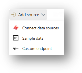
To get started, you need a data source that delivers events.
In terms of technologies, a wide range of options is supported. In addition to Microsoft services (e.g. Azure IoT Hub, Azure Event Hub, OneLake events), these also include Apache Kafka streams, Amazon Kinesis Data Streams, Google Cloud Pub/Sub, and Change Data Captures.
If none of these are suitable, you can use a custom endpoint, which supports Kafka, AMQP, and Event Hub. You can find an overview of all supported sources here.
Tip: Microsoft offers various “sample” data sources, which are great for testing and experimentation.
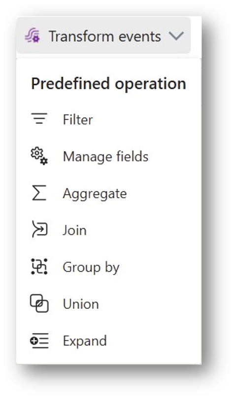
The incoming event data can now be cleansed and transformed in various ways. To do this, you append and configure one of several transformation operators after the source. These operators allow you to filter, combine, and aggregate data, select fields, and so on.
Example: Suppose the data source transmits the current room temperature multiple times per second, but for our planned analysis a one-minute granularity would be perfectly sufficient. So we use the “Group by” transformation to calculate the average, minimum, and maximum temperature for each 5-second window. This significantly reduces the data volume (and associated costs) before storage, while still preserving all the relevant information.
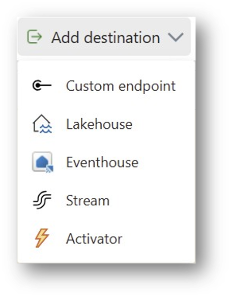
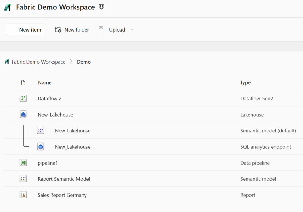
After all transformation steps are completed, the event data is sent to a destination. Most often, this is a table in an Eventhouse. The following destinations are supported:
Event streams also support multiple destinations. This is useful, for instance, when implementing a Lambda architecture: you store fine-grained data (e.g. on a per-second basis) in an Eventhouse for a limited time to support real-time scenarios. In parallel, you aggregate the data (e.g. per minute) and store the result in a Lakehouse for historical data analysis.
Using Eventstreams requires a paid Fabric Capacity. Microsoft recommends at least an F4 SKU (monthly prices can be found here). In practice, the adequate capacity level depends on several factors, particularly the needed compute power, data volume, and total Eventstreams run time. Further details can be found here.
If you don’t need an Eventstream for some time, you can deactivate it to avoid unnecessary load on your Fabric Capacity. This can be done separately for each source and destination.

Rupert Schneider
Fabric Data Engineer at scieneers GmbH
rupert.schneider@scieneers.de


In today’s business world, there is an increasing focus on basing decisions and processes on a solid foundation of data. The technical solution is usually a combination of data warehouses and dashboards that compile company data and present it in a visual format that is easy for everyone to understand and use.
Implementation often relies on batch processing, whereby data is collected and prepared automatically — for instance, once a day or less frequently, such as every hour or every few minutes.
This approach works well for many applications. However, it has its limitations when it comes to analysing information ‘in real time’ with a delay of a few seconds at most. Here are a few examples:
None of this is new, but previous solutions were often challenging to implement and required considerable expertise.
This is precisely where Microsoft stepped in: in 2024, the Fabric platform was expanded to include Real-Time Intelligence and various building blocks that can be used to bypass much of the complexity and swiftly develop functioning solutions.
In future articles, we will closely examine the most important of these ‘fabric items‘. Here is a brief overview:

Eventstream
Event streams continuously receive real-time data (events) from various sources. This data is transformed as required and ultimately forwarded to a destination responsible for storing it. Typically, this destination is an event hub. No code is required.

Eventhouse
An event house is an optimised data storage facility designed specifically for events. It contains at least one KQL database, which stores event data in table form.

Real-Time Dashboard
Real-time dashboards are similar to Power BI reports, but they are a standalone solution independent of Power BI. A real-time dashboard contains tiles with visualisations, such as diagrams or tables. These are interactive, and you can apply filters, for example. Each visual retrieves the necessary data via a database query formulated in KQL (Kusto Query Language), typically from an event hub.
Activator
Activator enables you to automatically perform an action based on certain conditions, such as a real-time dashboard or a KQL query. The simplest action is sending a message via email or Teams, but you can also trigger a Power Automate flow.
So what do I need to learn to implement a solution with Real-Time Intelligence?,
It essentially boils down to KQL and a basic understanding of the aforementioned fabric items. A lot of it is no-code. KQL is less common than SQL, but the basics are easy to learn, and feel natural after a short time.
We’ll be back soon with more posts on Fabric Real-Time Intelligence in our blog, delving deeper into the various topics.
Rupert Schneider
Fabric Data Engineer at scieneers GmbH
rupert.schneider@scieneers.de
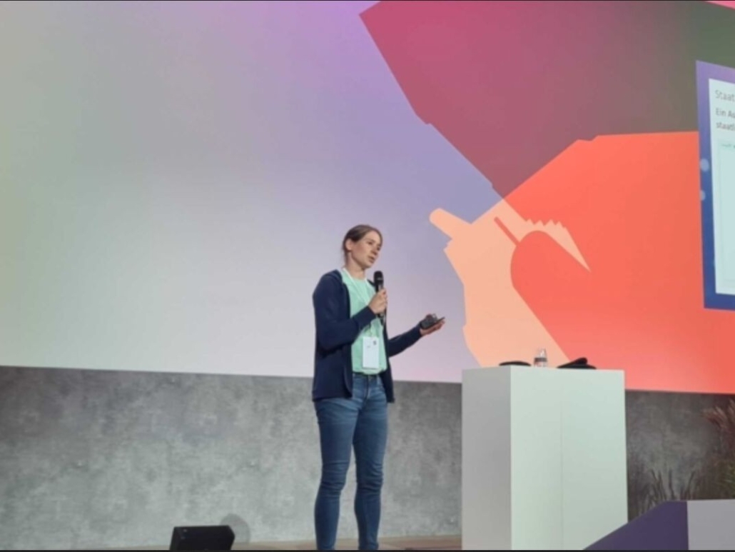
At this year’s Minds Mastering Machines (M3) conference in Karlsruhe, the focus was on best practices for GenAI, RAG systems, case studies from different industries, agent systems, and LLM, as well as legal aspects of ML. We gave three talks about our projects.

Global models such as TFT and TimesFM are revolutionising district heating forecasting by providing more accurate predictions, using synergies between systems and effectively solving the cold start problem.

Is the CI/CD pipeline taking forever? Is it taking too long to build a container image locally? One possible reason could be the size of container images – they are often unnecessarily bloated. This article presents several strategies to optimise images and make them faster and more efficient. 🚀
A grown project with numerous dependencies in pyproject.toml can quickly become confusing. Before taking the next step – containerization with Docker, for example – it is worth first checking which dependencies are still needed and which are now obsolete. This allows you to streamline the code base, reduce potential security risks, and improve maintainability.
One option would be to delete all dependencies and the virtual environment and then go through the source code file by file to add only the dependencies that are needed. The command line tool deptry offers a more efficient strategy. It takes over this tedious task and helps to quickly identify superfluous dependencies. The installation is carried out with
uv add --dev deptry
The analysis of the project can then be started directly in the project folder with the following command
deptry .
After that, deptry lists the dependencies that are no longer used
Scanning 126 files...
pyproject.toml: DEP002 'pandas' defined as a dependency but not used in the codebase
Found 1 dependency issue.
In this case, pandas no longer appears to be used. It is recommended to check this and then remove all dependencies that are no longer needed.
uv remove deptry pandas
If you are using a package such as pytorch, docling, or sparrow with torch(vision) as a dependency and only want to use the CPU, you can omit the installation of the CUDA libraries. This can be achieved by specifying an alternate index for torch(vision), where uv will look for the package first, with no dependencies on the CUDA libraries for torch(vision) defined in this index. To do this, add the following entry to pyproject.toml under dependencies.
[tool.uv.sources]
torch = [
    { index = "pytorch-cpu" },
]

torchvision = [
    { index = "pytorch-cpu" },
]


[[tool.uv.index]]
name = "pytorch-cpu"
url = "https://download.pytorch.org/whl/cpu"
This is what the images look like with and without the alternative index:
REPOSITORY           TAG       IMAGE ID       CREATED              SIZE
sample_torchvision   gpu       f0f89156f089   5 minutes ago        6.46GB
sample_torchvision   cpu       0e4b696bdcb2   About a minute ago   657MB
With the alternative index, the image is only 1/10 as large!
Whether the Python project is just starting or has been around for a while, it is worth having a look at the sample docker files provided by uv: uv-docker-example.
These provide a reasonable base configuration and are optimised to create the smallest possible images. They are extensively commented and use a minimal base image with Python and uv preinstalled. Dependencies and the project are installed in separate commands, so that layer caching works optimally. Only the regular dependencies are installed, while dev dependencies such as the previously installed deptry are excluded.
In the multistage example, only the virtual environment and project files are copied to the runtime image, so that no superfluous build artefacts end up in the final image.
This tip will not reduce the size of the image, but it may save you some headaches in an emergency.
When deploying the Docker image in an Azure WebApp, /home or underlying paths should not be used as WORKDIR. The /home path can be used to share data across multiple WebApp instances. This is controlled by the environment variable WEBSITES_ENABLE_APP_SERVICE_STORAGE. If this is set to true, the shared storage is mounted to /home, which means that the files contained in the image are no longer visible in the container.
(If the Dockerfile is based on the uv examples, then the WORKDIR is already configured correctly under “/app”.)

Almost every company conducts research and development (R&D) to bring innovative products to market. The development of innovative products is inherently risky. As they are products that have never been offered, it is usually unclear whether and to what extent the desired product features can be realized and how exactly they can be realized. The success of R&D therefore depends largely on the acquisition and use of knowledge about the feasibility of product features.
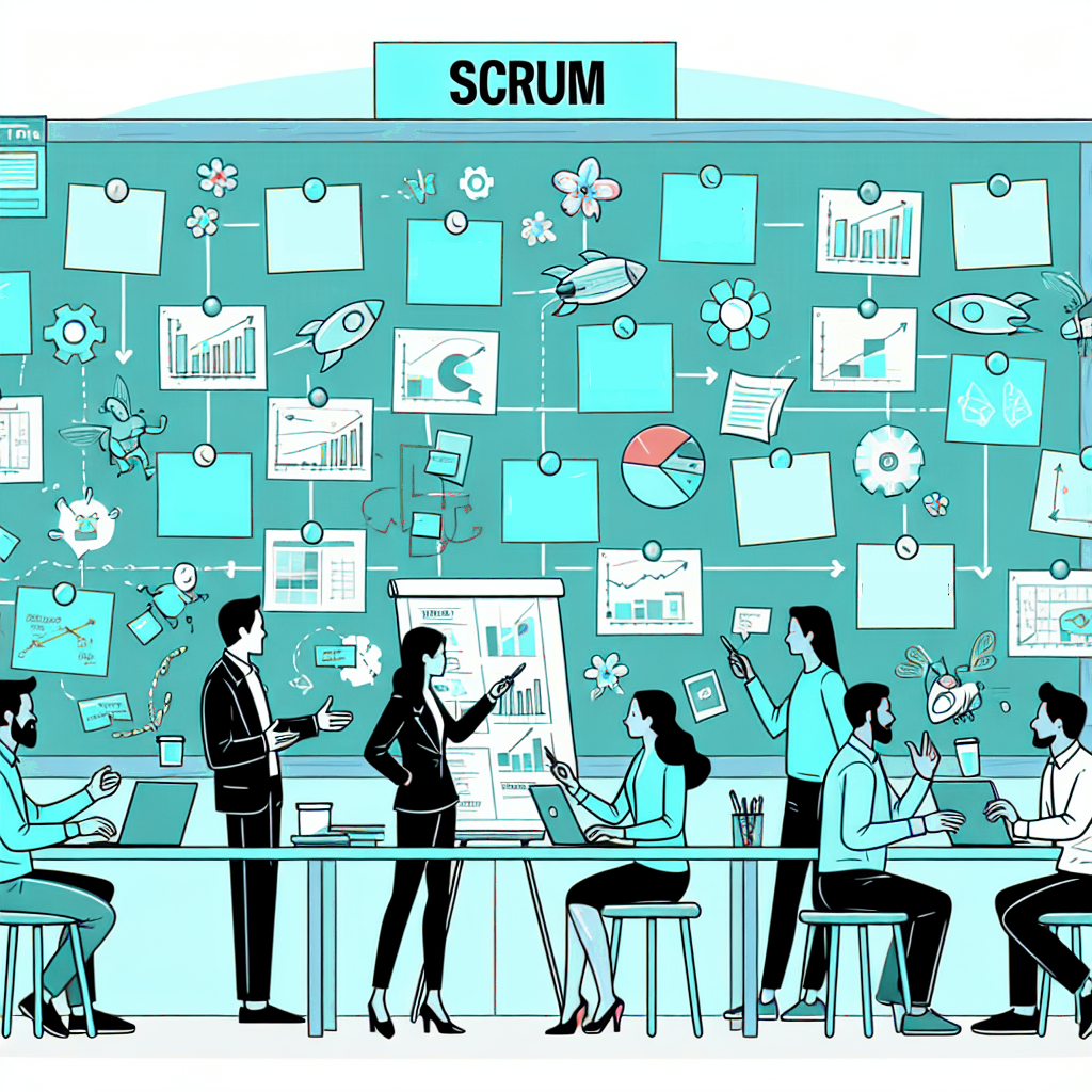
Scrum is by far the most popular form of agile project management today1. Some of the key features of Scrum are constant transparency of product progress, goal orientation, simple processes, flexible working methods, and efficient communication. Scrum is a flexible framework and contains only a handful of activities and artefacts2. Scrum deliberately leaves open how Backlog Items (BLIs) are structured, what the Definition of Done (DoD) of BLIs is, and how exactly the refinement process should work. A Scrum team has to manage these aspects itself. This flexibility is another reason why Scrum is so successful: Scrum is used in various domains, supplemented with domain-specific processes or artefacts3.
Scrum is also well established in R&D4. As described above, the success of an R&D Scrum team depends on how efficiently the team acquires and uses knowledge. In Scrum, so-called spikes have become established for knowledge acquisition. Spikes are BLIs in which knowledge about the feasibility and cost of product features is gained without actually realising the features. In this article we want to show what is important when implementing spikes in Scrum and how a Scrum team can ensure that the knowledge gained from spikes is used optimally. We illustrate these good practices with concrete examples from 1.5 years of Scrum in a research project with EnBW.
– – – – – – – – – – – – – – – – – – – – – – – – – – – – – – – – – – – – – – – – – – – – – – – – – – – – – – – – – – – – – – – – – – – – – – – – – – – – –
A widely used method for gaining knowledge in Scrum is called spikes – BLIs, where the feasibility and effort of product features are assessed without realizing the features. The idea of spikes comes from eXtreme Programming (XP)5.
Acquiring knowledge through spikes serves to reduce excessive risk6. The proportion of spikes in the backlog should, therefore, be proportional to the current risk in product development. In an R&D Scrum team, there may be many open questions and risks, and spikes may account for more than half of a sprint, as in the Google AdWords Scrum team7. However, an excessive proportion of spikes inhibits a team’s productivity because too much time is spent gaining knowledge and too little time is spent implementing the product8. Prioritizing spikes over regular BLIs is an important factor for the success of R&D Scrum projects.
Another important factor is the definition of quality criteria for spikes. Specifically, a Scrum team can establish a Definition of Ready (DoR) and a Definition of Done (DoD) for spikes. The DoR defines what criteria a spike must meet to be processed; the DoD defines what criteria a spike must meet to be done. Both definitions influence the quality and quantity of the generated knowledge and its usability in the Scrum process. The DoD is a mandatory part of Scrum. On the other hand, the introduction of a DoR is at the discretion of the Scrum team and is not always useful9.
The reason for a spike is almost always an acute and concrete risk in product development. However, the lessons learned from a spike can be valuable beyond the specific reason for the spike and can help inform product development decisions in the long term. To have a long-term effect, the team needs to store the knowledge gained from spikes appropriately.
The use of spikes in R&D projects therefore raises at least three questions:
The literature on Scrum leaves these questions largely unanswered. In a multi-year R&D research project with EnBW, we applied various answers to the questions and gained experience with them. We developed two good practices in the process, which we present in this blog post: (1) a regular interval for “spike maintenance,” i.e., for sharpening concrete hypotheses in spikes, and (2) a lightweight lab book for logging findings. We also supplement the two practices with a suitable DoR and DoD.
– – – – – – – – – – – – – – – – – – – – – – – – – – – – – – – – – – – – – – – – – – – – – – – – – – – – – – – – – – – – – – – – – – – – – – – – – – – – –
Refinement is an ongoing activity of the whole Scrum team. BLIs from the backlog are prepared for processing: BLIs are reformulated, divided into independent BLIs and broken down into specific work steps. Many Scrum teams use regular intervals to refine and gain a common understanding of the backlog.
In our experience, collaborative refinement is a common source of spikes. This is because unresolved issues and risks come to light when the team discusses the backlog. Unresolved risks in a BLI often manifest in the team’s difficulty defining a concrete DoD and the wide variation in team members’ estimates of the effort involved. Specific phrases used by team members may also indicate risks, e.g.:
Once a risk has been identified, the team must decide whether it is so great that it should be reduced with a spike. The spike is then created in the backlog as a BLI draft. To not exceed the regular refinement deadline, we recommend that newly created spikes are not refined and prioritized in this deadline. Instead, we recommend that the team meet regularly one to two days after the regular refinement to perform “spike maintenance.” In the meantime, spike drafts can be assigned to individual team members to prepare for the spike maintenance interval, e.g., by collecting concrete hypotheses and ideas for experiments.
Of course, spikes can also be created outside of a joint sharpening appointment, e.g., when performing a BLI. Even then, it is a good idea to collect the spikes as drafts and then sharpen them at the next spike maintenance interval. This way, the spike events are not forgotten but do not lead to scope creep in the current sprint.
During the spike maintenance interval, the collected spikes must be refined and prioritized in the backlog. In our experience, most spikes are directly related to one or more BLIs – the BLIs whose implementation poses acute risks. In this case, prioritization is simple: use the existing prioritization of BLIs and add each spike to the list before its associated BLI.
– – – – – – – – – – – – – – – – – – – – – – – – – – – – – – – – – – – – – – – – – – – – – – – – – – – – – – – – – – – – – – – – – – – – – – – – – – – – –
We suggest a light lab book to store the knowledge gained from the spikes. The lab notebook documents the following aspects for each spike in 1-2 sentences.
Completeness and compression are crucial for the long-term added value of the lab notebook. Completeness means that the results of all spikes end up in the lab book; compression means that only the essential results and consequences for the project are briefly and concisely recorded in the lab book. In this quality, the lab book can be used as a discussion reference.
In the project with EnBW, we implemented the lab book as a wiki page in the team’s project wiki. We sorted the entries on the page in descending chronological order, i.e., the knowledge from the current spikes was at the top. We used the lab book for about a year and noticed no scaling problems. The lab book was highly regarded as a source of knowledge within the team and was regularly used in discussions.
– – – – – – – – – – – – – – – – – – – – – – – – – – – – – – – – – – – – – – – – – – – – – – – – – – – – – – – – – – – – – – – – – – – – – – – – – – – – –
This brings us to our final recommendation: a concrete definition of the DoR and DoD for spikes, in line with the two previous good practices.
The DoR specifies which criteria spikes must fulfil before they can be included and worked on in a sprint. As mentioned, the DoR is not part of Scrum, but a commonly used extension. Some Scrum experts are critical of the DoR because it can lead to important BLIs not being included in a Sprint for “aesthetic reasons”10. We, therefore, propose a compromise: important BLIs are always included in the next sprint, but the person working on the BLI is responsible for ensuring that the BLI fulfills the DoR before it is worked on. This means fulfilling the DoR criteria is the first step of any BLI.
Our DoR proposal for spikes is simple: before a spike is processed, the lab book entry for the spike must be filled in as precisely as possible. In particular, the hypotheses to be investigated must be listed. In the EnBW team, we have had good experience with one team member formulating the hypotheses before working on the spike and then having them critically reviewed by another team member. Once the hypotheses are complete, understandable, and clearly defined, work on the spike can begin.
The lab book entry provides a framework for the spike. This is similar to the well-known Test-Driven Development (TDD) in software development. Unit tests are first used to define what the software should do, and then it is implemented. The creation of a lab book entry before each spike could be described by analogy as hypothesis-driven learning (HDL): first, hypotheses are used to define what is to be learned, then the hypotheses are tested.
The analogy between TDD and HDL is also useful in describing the advantages of HDL. Just as TDD provides a constant incentive to reduce software complexity, HDL provides an incentive to keep experiments simple and focused. And just as the programmed tests in TDD replace much of the written documentation of software, the lab book entries in HDL replace much of the written documentation of knowledge from spikes.
A spike’s DoD is at least as important as its DoR. It determines what criteria must be met for the spike to be completed. The spike’s lab book entry can also determine these criteria. Specifically, we propose that a spike is complete when all hypotheses listed in the lab notebook entry have been confirmed or rejected, the lab notebook entry has been written, and the results have been communicated to the team.
– – – – – – – – – – – – – – – – – – – – – – – – – – – – – – – – – – – – – – – – – – – – – – – – – – – – – – – – – – – – – – – – – – – – – – – – – – – – –
In this blog post we have made a concrete proposal on how to use spikes in R&D Scrum projects. Our proposal enables an R&D Scrum team to assess the feasibility of innovative product features – in time before the product is implemented and with reasonable effort.
At the core of our proposal are two good practices that have proven successful in our own R&D Scrum projects: first, a spike maintenance interval, and second, a lightweight lab book for logging findings. We have shown how both practices can be integrated into Scrum using a simple DoR and DoD.
With the two good practices we fill a gap in the Scrum literature: there are hardly any concrete practices for the creation, prioritisation, quality assurance and long-term use of spikes. The proposed good practices are simple and general enough to be applicable and useful for most R&D Scrum teams. We would be happy if other Scrum teams could be inspired by them.

Moritz Renftle
Data Scientist at scieneers GmbH
moritz.renftle@scieneers.de
Microsoft Fabric is a versatile and powerful platform for today’s data and analytics requirements and is currently attracting a lot of attention from our customers. It meets a wide range of needs, depending on the size of the organisation, its data culture and its development and analysis focus.
Customers in the Power BI environment are particularly benefiting from the extension of the self-service approach: Using familiar web interfaces and without specialised development tools, business departments or end users can quickly get started with data preparation.
Experienced developers and IT teams, on the other hand, want to ensure that they can continue to use best practices in Fabric, such as development in an IDE, version management with Git, or established testing and rollout processes. This raises the question of how to robustly test and deploy key changes to a large number of users.
In this blog post, we aim to provide an overview of the development and collaboration capabilities and deployment scenarios in Fabric. Although we try to provide a general overview, Microsoft is working to develop new features and enhancements for Fabric, so technical details may change over time. For the latest information on Fabric, see the official documentation or visit the Microsoft-Fabric-Blog.
Fabric as Software-as-a-Service is usually operated directly via the browser.
If you are already familiar with the Power BI service, the familiar workspace concept will help you get up and running quickly. New fabric objects, such as data flows or pipelines, can be easily created and edited in the web interface – no local development environment or additional software installations are required.
Another key advantage of browser-based development in Fabric is its cross-platform usability on Windows and MacOS. However, browser-based development environments tend to be less flexible and customisable than an integrated development environment (IDE), with a limited set of tools and integration options. Fabric is no different.
Changes to Fabric objects are instantly live and can be seen and tested by other users, significantly accelerating development cycles. However, there are risks associated with this immediate visibility: errors or unwanted changes immediately affect all users and cannot be undone as easily as with locally stored files.
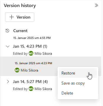
For this reason, Microsoft is working on integrated versioning, including rollback functionality for various Fabric objects. This is already available for notebooks and is currently in Preview-Phase for semantic models.
Despite some limitations in flexibility and tool integration, the web interface provides a quick and convenient introduction to development and simplifies collaboration in distributed teams. For example, the notebook GUI supports parallel working, including comments and cursor highlighting, which facilitates pair programming, remote debugging and tutoring scenarios.
This development process is particularly suitable for scenarios where isolated development is not required and changes can be made directly to the live version – for example, for end users in non-technical departments or less critical use cases.
On the other hand, if a dedicated environment is required to test new features or customisations without affecting the live version, there are two basic approaches.
Client tools are available for various Fabric objects that can be installed on a computer and used to edit these objects locally. In most cases, a local copy of the Fabric object is created, edited, and uploaded back to the Fabric workspace once all changes have been made.
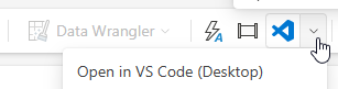
Power BI users are already familiar with this process: A Power BI report from Fabric can be downloaded as a .pbix file and edited locally using Power BI Desktop. The changes to the report are not visible in Fabric until the local changes are published. Fabric notebooks can be edited in a similar way; they can be exported as an .ipynb file and edited locally with your preferred development tools. There is an extension to VS Code (currently called “Synapse”) that simplifies this process.
Once you have installed this VS Code extension, you can create a local copy of the notebook directly from a button in the Fabric GUI and open it in VS Code.
This allows you to work in a familiar development environment. If required, you can even run the code on the fabric capacity via the fabric-spark-runtime and thus process large amounts of data. As soon as all changes have been made to the notebook, the customized version is simply uploaded backto the Fabric Workspace via the VS Code plugin – including a practical diff function to display differences compared to the version in the Fabric Workspace.
The Fabric environment can also be accessed in other areas with local tools. For example, VS Code or SQL Server Management Studio can be used to write SQL queries or define views. The Fabric Warehouse in particular is currently well integrated into these tools, but a connection is generally possible with all SQL-based fabric objects.

These features can be used without connecting the Fabric workspace to a Git repository. This makes the process particularly suitable for users who need an isolated development environment but are new to Git, or whose workspaces are not (yet) connected to a Git repository for organisational reasons.
For experienced developers, however, Git integration is a key component of professional development processes. For this reason, Microsoft Fabric also offers native integration with Azure DevOps and GitHub.
Microsoft Fabric allows you to connect a workspace to an Azure DevOps or GitHub repository to use a Git-integrated development process, such as versioning. A detailed explanation of this functionality’s features and limitations can be found here.
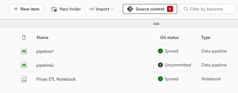
When a workspace is connected to a repository, the Git status of each fabric object can be viewed at any time. Changes to objects or the creation of new objects can be committed directly from the GUI and saved to the repository. This ensures that accidentally deleted items can be recovered at any time.
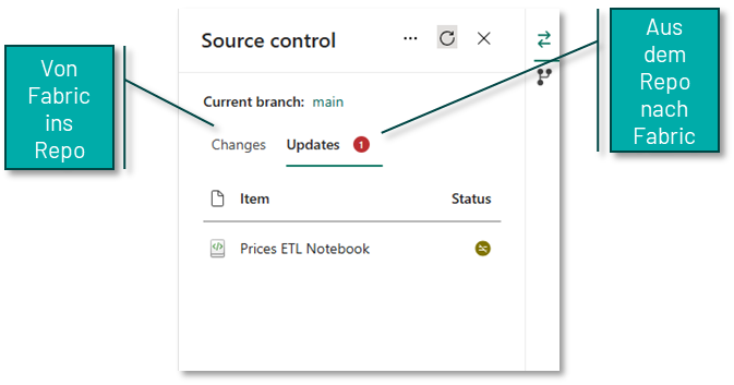
It is important to understand that this synchronisation between Fabric and the repository can work in both directions. This means that changes from Fabric can be saved to the repository and changes to the objects in the repository (e.g. if a notebook has been edited directly in the repository) can be imported back into the Fabric workspace.
If the Fabric workspace is Git-integrated, this opens up further possibilities for working locally with different Fabric elements. By cloning the relevant repository, you can use all the familiar Git features, such as local feature branches or individual commits for important intermediate states.
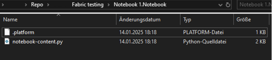
The downside is that the individual Fabric items in the repository are stored in formats that are primarily designed for Git-optimised storage rather than convenient editing. Notebooks, for example, are not saved as .ipynb files but as pure .py files, supplemented by an additional platform file containing important metadata. This can make it difficult to work locally with branches in the repository.
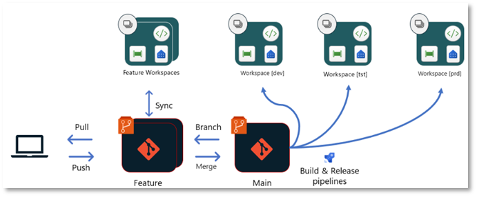
To achieve an isolated development environment, you do not necessarily need to use local tools in Fabric. Provided the workspace is Git-integrated, Fabric also offers native options. Of particular interest is the ability to branch to a new feature workspace, which is described in more detail here.
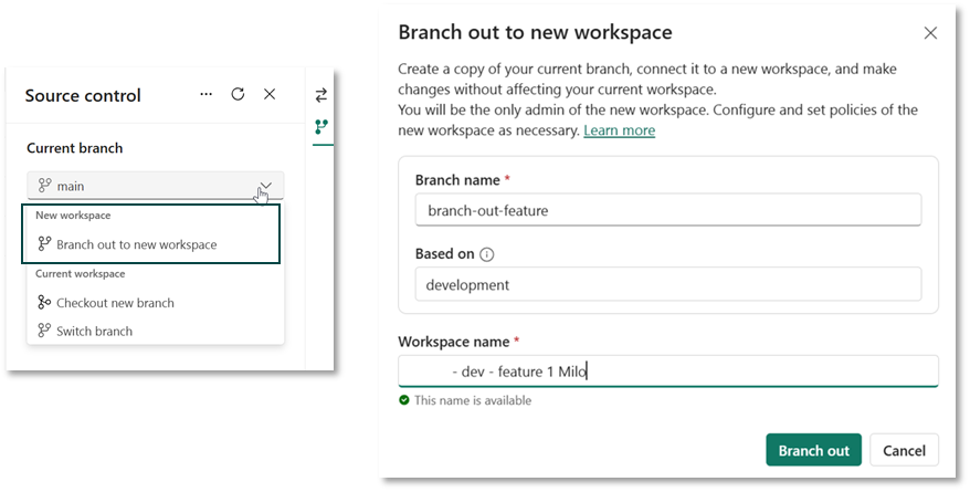
When you use this feature, a copy of the workspace is created to which only you have access. In this copy, you can develop in isolation, without affecting the functionality of the objects in the real workspace. The following happens in the background
A new empty workspace with the defined name is created.
The contents of the current workspace are copied to this branch.
A new branch is created in the repository, the name of which can also be defined.
The Tissue objects are created in the newly created workspace based on the newly created branch.
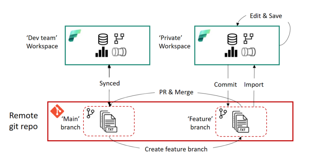
You can now work on the fabric objects in isolation and commit the changes to the new branch, for example if you want to continue developing a notebook. It is important to note that data (e.g. in a lake house) is not stored in the repository and is therefore not available in the new workspace. This means that a notebook will still connect to the lakehouse in the current workspace if it was used as a data source in the notebook.
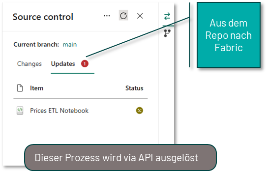
Once you have made all the changes in the feature workspace, you still need to commit those changes back to the actual workspace. This process primarily takes place in Azure DevOps or GitHub and requires a basic understanding of Git. A pull request (PR) is created to merge the feature branch into the main branch of the actual workspace. All the usual DevOps and GitHub features are available here, such as tagging reviewers. Once the PR has been successfully completed, the main branch in the repository has a more up-to-date status than the fabric objects in the workspace itself. Finally, the status needs to be transferred from the repository to the workspace. To do this, you can use the update process described above in the source control panel of the fabric workspace, or you can automate this process via API.
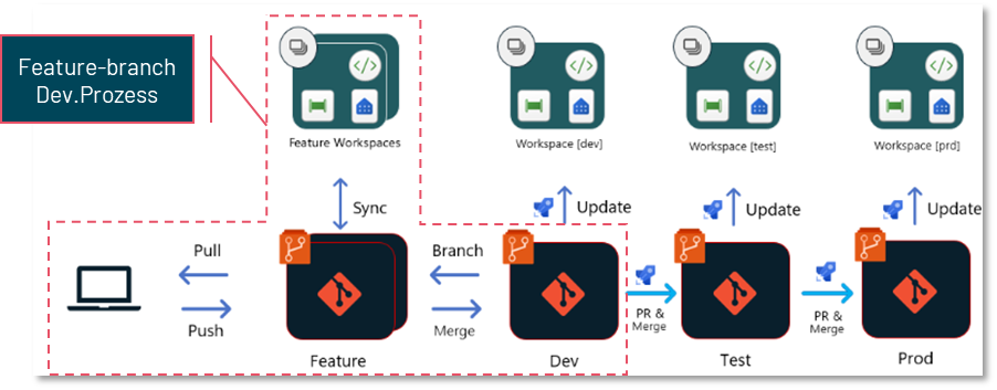
The following diagram illustrates the process.
This development process offers the full benefits of Git-based development and can be supplemented with local client tools if required. For example, it is possible to open the notebooks in the feature workspace using the process described above in VS Code.
However, there are some drawbacks to this process. Since pull requests and merges are done in Azure DevOps or GitHub, this process requires experience using Git and Azure DevOps or GitHub. In addition, users wishing to use this feature in Fabric must be authorised to create workspaces, which must first be approved by an administrator. At the moment, feature workspaces are also not automatically deleted after a successful merge with the source workspace. This can result in workspaces that are no longer needed accumulating over time unless they are manually deleted.
A further step in professionalising the use of Microsoft Fabric is to run workloads in multiple environments. Typically, a distinction is made between a development environment (Dev.) and a production environment (Prod.). This allows the workload in the development environment to be developed in isolation and iteratively, while the end users in the production environment always have a working and well-documented version of the workload.
Once a satisfactory point in the development process is reached, the development state is transferred from the development environment to the production environment. This is known as the deployment process. Microsoft Fabric provides several options for this.
The easiest way to integrate a deployment process into Fabric is to use Fabric Deployment Pipelines. They are an integral part of Fabric and require no additional tools – the development workspace does not even need to be connected to a Git repository to use them.
A workspace is created for each environment, and then a deployment pipeline is set up in the development workspace. A simple interface is used to define which Fabric objects to move from the source workspace (Development in the figure below) to the target workspace (Test in our case), and click ‘Deploy’.
As different environments tend to have different properties – for example, the database they access – Deployment-Rules can be defined for each Fabric object. These ensure that these properties are adjusted accordingly during the deployment process.
However, these deployment rules cannot yet be used for all Fabric objects and only support a pre-defined selection of properties that can be customised. For example, it is not possible to replace parameter values previously defined in code in a fabric notebook.

Overall, Fabric Deployment Pipelines provide an easy entry point to multi-environment development without requiring in-depth Git experience. They are particularly suited to workloads managed by non-technical departments, for example, and are a logical extension of the self-service principle.
The second way to implement a deployment process in Fabric requires that all workspaces representing a particular environment (e.g. Dev, Test and Prod) are linked to different branches of the same Git repository. The functionality of branch-based deployment is similar to the feature branch development process characterised in the following diagram. In principle, however, the branch-based deployment process can be combined with any development process as long as a Git integration is set up.
This process uses the functionality of Azure DevOps Pipelines (or GitHub Actions), which automatically react to changes in repository branches and can trigger specific processes.
Once a new development state has been created in the development environment (Dev.) and is ready for deployment, a pull request (PR) is created in a test branch in the repository. Reviewers can review and approve the new changes in this branch.
Once the test branch is released and updated, a DevOps pipeline is automatically started to perform various actions on the object definitions in that branch. This pipeline can, for example, adjust environment parameters (such as database connections), run automated tests on the code, or ensure that the code adheres to style and naming conventions.
The customised code is then stored in another branch, such as Test-Release. This test-release branch is connected to the test workspace in Fabric. A second pipeline responds to updates to this branch and uses an API to ensure that the status of this branch is transferred to the Fabric workspace.
Further testing, such as data quality testing, can then be performed directly in Fabric in the test workspace before the code is moved to the production workspace in an analogous process.
In addition to an understanding of Git, this form of deployment process requires experience in setting up Azure DevOps pipelines or GitHub actions, and is therefore designed for experienced developers and critical workloads. However, using professional deployment tools then provides full flexibility to design the deployment process and integrate advanced steps such as code testing.
Working with dedicated branches per environment also makes it easy to manage different versions in each environment and roll back to previous versions quickly.
Another way of deploying in Fabric is not to connect each workspace directly to a branch in a repository using the built-in options, but to deploy directly to each workspace from a shared master branch using Build- und Release-pipelines.
In this approach, as in the previous process, a build pipeline can exchange environment parameters (such as database connections) depending on the target environment, perform automated tests on the code, or ensure that the code conforms to style and naming conventions. In this approach, the result is not stored in a separate branch, but is passed as an artifact to, for example, a release pipeline. This then uses the Fabric Item API to deploy the relevant Fabric objects or changes to the target workspace.
Libraries such as the fabric-cicd Python Library can be used to simplify interaction with the Fabric API.
As with branch-based deployment, this approach requires experience with Azure DevOps pipelines, but also allows full flexibility in the exact design of the deployment process.
In this article, we have presented examples of the most common development and deployment processes in Microsoft Fabric. However, especially for the deployment processes via Azure DevOps or Github, there is of course full flexibility in the concrete design to adapt these exactly to your own needs. It is also not necessary to choose a single development or deployment process for all workloads to be mapped to Fabric. The choice of process should always be tailored to the specific requirements and workload. For example, a professional deployment process may be appropriate for central data products, such as an enterprise-wide data warehouse, while deployment via deployment pipelines may be sufficient for individual departments, or deployment processes may not be required at all.
If you want to learn more tips and tricks about Microsoft Fabric, feel free to take a look at our Microsoft Fabric Compact Introduction workshop!

Milo Sikora
BI Consultant at scieneers GmbH
milo.sikora@scieneers.de
Disseminators of disinformation use various strategies to make false statements appear authentic. To combat this effectively and reduce the credibility of such disinformation, it is crucial that those affected not only recognize it as such but also see through the misleading rhetorical strategies used.
Today, this is more important than ever: we are bombarded with information and opinions daily on social media or at family gatherings. We often decide whether to accept them as valid or questionable in fractions of a second. Knowledge of commonly used rhetorical strategies strengthens intuition and encourages critical questioning of dubious arguments.
This is why we have developed the DesinfoNavigator – a tool that helps people recognise and refute disinformation. With the DesinfoNavigator, users can check text excerpts for misleading rhetorical strategies and at the same time receive instructions on how to examine the text passages for these strategies.
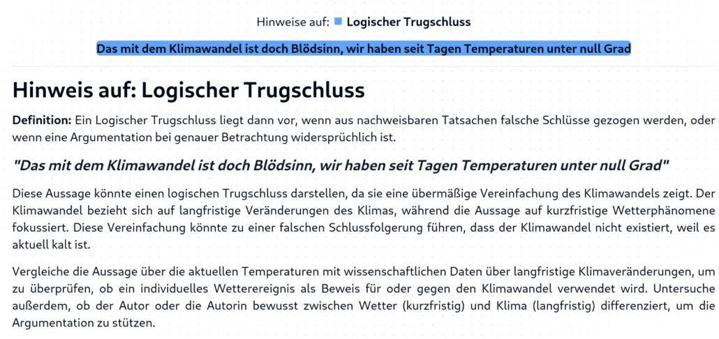
In order to analyse these strategies, the DesinfoNavigator uses the PLURV-Framwork, which includes the following five categories Pseudo-expert:s, Logical Fallacies, Unfulfilled Expectations, Cherry-Picking and Conspiracy Myths.
In its technical implementation, the DesinfoNavigator uses a large language model (LLM). In a first step, the tool analyses the user input for possible rhetorical strategies according to the PLURV framework. In addition to the user input, the language model also receives a detailed description of the strategies, including examples. As a result, the model provides text passages that contain references to one of the strategies. In the second step, the language model generates an action instruction for each identified text passage, which provides instructions on how to check the text passage with regard to the strategy.
It is important to emphasise that the DesinfoNavigator does not perform classical fact-checking, but analyses whether and which rhetorical strategies can be used in a text. We therefore see the DesinfoNavigator as a logical complement to existing fact-checking tools.
To achieve the greatest possible social benefit, we have decided to make the DesinfoNavigator free and freely accessible. This will allow a wide audience to actively participate in detecting and combating disinformation. Curious?
You can currently try out the DesinfoNavigator at https://desinfo-navigator.de/. We look forward to receiving helpful feedback and interested partners who want to help us develop the tool further.


Communication scientist with a research focus on disinformation
Clara Christner (ResearchGate)
Dr. Clara C. (LinkedIn)

Welcome to scieneers.
When choosing an employer today, it’s not just about the job itself but also about the values and benefits the company can offer.
It is important to us that our employees not only find a job, but also an environment in which they can thrive and develop.
We are committed to creating a working environment that fosters both professional and personal development.
Our benefits are designed to offer the best of both worlds. A culture that focuses on transparency, inclusion and sustainability, and benefits that inspire and are a reason to join our team.
Here is an overview of the benefits you can expect when you join us:
We understand the importance of flexibility in the workplace. We trust our people to know best when and where they can be productive.
Whether you want to work in a modern office or in the peace and quiet of your own home, we can accommodate both.
We have three beautiful, well-connected offices in Hamburg, Cologne and Karlsruhe.
We also offer a wide range of home office options to enable our employees to organise their working day in a way that best suits their individual lifestyle.


Family is important to us too.
That is why we want to help our employees balance family and career.
In addition to flexible working hours, we also offer support for children’s daycare. In this way, we want to make combining work and family life easier.


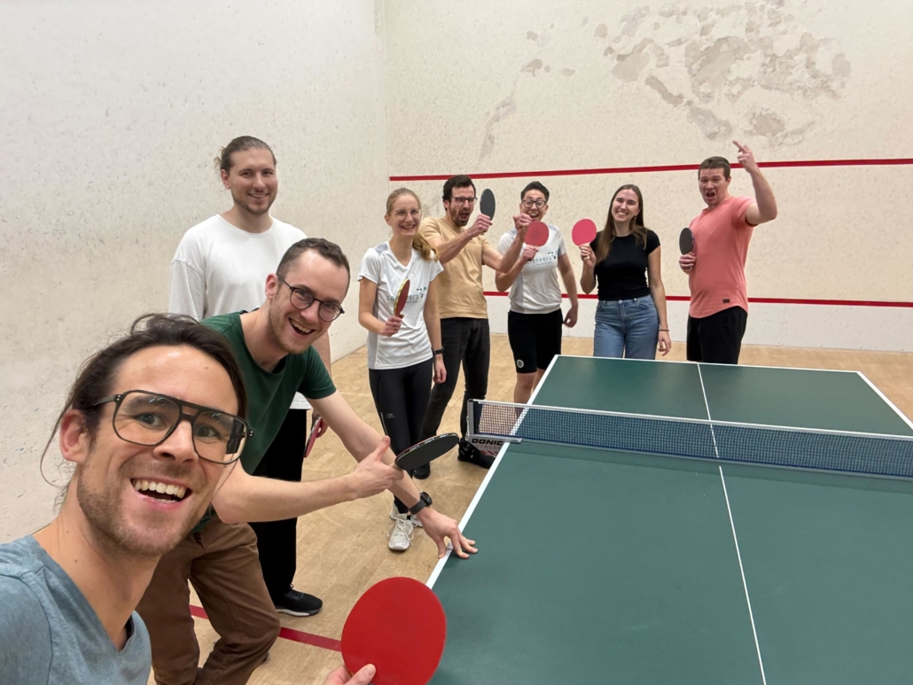
Whether it’s eating together, sporting activities or cultural experiences, our aim is to create a working environment that focuses on team spirit and interaction between our team members.
With regular team events, office lunches, and other joint activities, we actively encourage communication and strengthen team cohesion.
We also like to celebrate successes and festivities together – our employees look forward to our regular get-togethers at different locations and our annual Christmas party.


The technology industry is fast-moving, so personal development is a crucial factor. That is why we offer every employee an individual training budget, which they can invest freely in their own development – be it books, online courses, training or their own ideas.
Of course, personal development is not limited to professional skills. We have a mentoring program to help new employees find their feet quickly. We also provide long-term support through regular feedback sessions and annual reviews.

Success is a shared project, and our employees make it possible. Through employee share ownership, we ensure that their commitment pays off in the long term and that they benefit directly.
Together with our employees, we are building a secure future. We think ahead and provide financial support for company pensions.

Mac, Windows or Linux – our employees can choose the hardware they want to work with. Of course, an up-to-date smartphone with a Telecom contract is also part of the standard equipment.
Our employees can also use the modern hardware of their choice for personal use. We make sure they have everything they need to be productive and creative.

Mobility is made easy with the Job-Ticket, job bike rental, or our company car leasing scheme – we help all employees to be mobile and sustainable in their travel. However, they choose to get to work.
We support all employees who are interested in staying active with a sports subsidy for membership of Urban Sports Club.

At scieneers, we believe in an open corporate culture where everyone is welcome. Inclusion, transparency and sustainability are values we actively live by.
We create a working environment that celebrates diversity and gives everyone a voice. That is why, as a company, we have signed the Diversity Charter (Charta der Vielfalt).


Our benefits are just part of what makes scieneers so special.
If you are looking for an open and modern company culture that supports and encourages you, then we want to hear from you
Discover our current job positions and find out how you can join us!